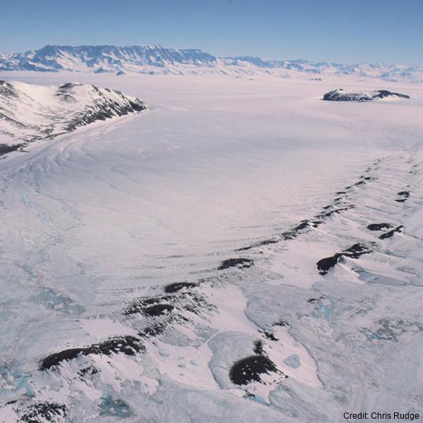
Plot data Mc Nemar: To enable comparisons with the 1961 and 2004 survey results, the Lambert Conformal Conic projection from the 2004 survey was used to precisely georeference and trim the RGB image across a 1-m2 grid, generating a total of 3,458 1-m2 grid cells. For each grid cell moss, lichen, or algae/cyanobacteria cover was extracted as one of the four cover classes: Heavy (>40%), Patchy (10–40%), Scattered (less than 10%), and None (0%) for the survey years 1962, 2004 and 2018. Ground truthing: To test the overall accuracy of cover classifications and ensure consistency with 2004 survey methodologies, a ground-truthing approach was performed. Photographs were taken of individual cells along eight transects, running west to east across the plot at 0.5, 1.5, 15.5, 16.5, 28.5, 29.5, 116.5 and 117.5 m distance from the NW corner. Each grid cell could be identified individually with an x/y coordinate in the centre and was surrounded by a rectangular frame parallel to the outer edge of the plot. A total of 174 photographs were taken and archived with Antarctica New Zealand. For each photographed grid cell, the presence of each functional group of vegetation and their cover class was assessed visually. Orthomosaic image: Aerial images were obtained using a DJI Matrice 600 Pro hex-rotor remotely piloted aircraft system equipped with a Canon EOS 5Ds camera (image size: 8688×5792 pixels, focal length: 50 mm, pixel size: 4.14 μm) on November 28, 2018. The flight altitude was 30 m above ground level, and a total of 10 ground-control points were included to provide accurate geo-referencing. An orthomosaic photo and accompanying DEM was generated with the acquired aerial images using Agisoft PhotoScan (now known as Metashape by Agisoft LLC, https://www.agisoft.com/) RELATED PUBLICATION: https://doi.org/10.1029/2022EF002823 GET DATA: https://doi.org/10.7488/ds/3417

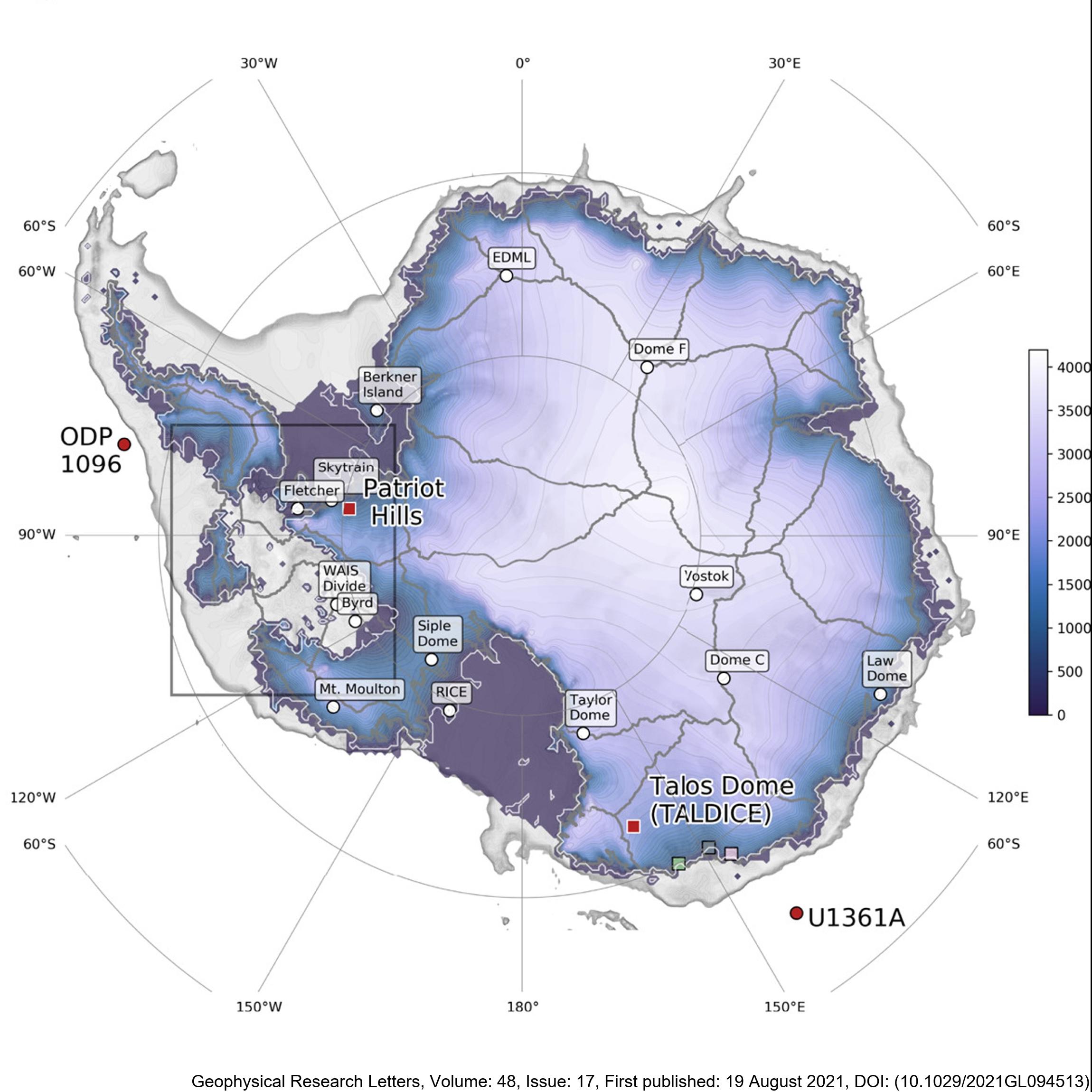
Here, we present new, transient, GCM-forced ice-sheet simulations validated against proxy reconstructions. This is the first time such an evaluation has been attempted. Our empirically constrained simulations indicate that the AIS contributed 4 m to global mean sea level by 126 ka BP, with ice lost primarily from the Amundsen, but not Ross or Weddell Sea, sectors. We resolve the conflict between previous work and show that the AIS thinned in the Wilkes Subglacial Basin but did not retreat. We also find that the West AIS may be predisposed to future collapse even in the absence of further environmental change, consistent with previous studies. There are two files, for Termination 1 ('T1') and Termination 2 ('T2'). They contain spatial fields for ice thickness, ice surface elevation, bedrock elevation, surface and basal velocity, and mask. The T1 outputs are every 500 years, whereas the T2 outputs are every 100 years. The spatial resolution of both is 20 km. Sea-level-equivalent mass loss can be calculated from these outputs, but is also provided here in a text file for convenience. RELATED PUBLICATION: Golledge, N.R., Clark, P.U., He, F., et al. (2021). Retreat of the Antarctic Ice Sheet During the Last Interglaciation and Implications for Future Change. Geophysical Research Letters, 48(17). https://doi.org/10.1029/2021GL094513 GET DATA: https://doi.org/10.17605/OSF.IO/GZB3H

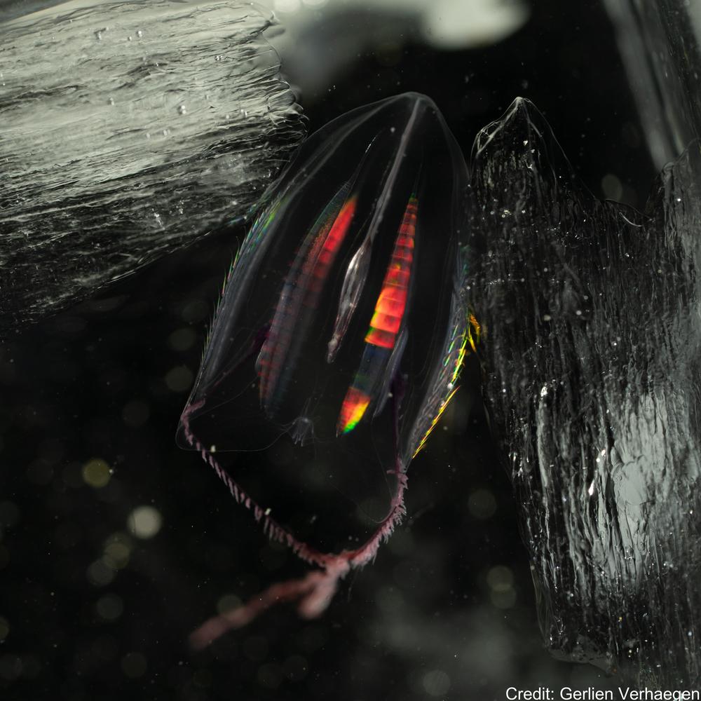
This Zenodo dataset contain the Common Objects in Context (COCO) files linked to the following publication: Each COCO zip folder contains an "annotations" folder including a json file and an "images" folder containing the annotated images. Verhaegen, G, Cimoli, E, & Lindsay, D (2021). Life beneath the ice: jellyfish and ctenophores from the Ross Sea, Antarctica, with an image-based training set for machine learning. Biodiversity Data Journal. https://doi.org/10.3897/BDJ.9.e69374 GET DATA: https://doi.org/10.5281/zenodo.5118012 GET DATA: http://ipt.pensoft.net/resource?r=life_beneath_the_ice-jellyfish_and_ctenophores_from_the_ross_sea_antarctica&v=1.3

This data publication contains biostratigraphic age events for the CIROS-1 drill core, updated age ranges for a suite of samples from the McMurdo erratics sample collection, age-depth tie points for CIROS-1, CRP-2/2A, DSDP 270, DSDP 274, ANDRILL 2A and ANDRILL 1B, and glycerol dialkyl glycerol tetraethers (GDGTs) abundances and indices for samples from the McMurdo erratics, CIROS-1, CRP-2/2A, DSDP 270, DSDP 274, ANDRILL 2A, and ANDRILL 1B. All sample sites are in the Ross Sea region of Antarctica. The McMurdo erratics are glacial erratics collected in the McMurdo Sound region between 1991 and 1996 (Harwood and Levy, 2000). The CIROS-1 drill core was collected from McMurdo sound in 1986 with samples spanning the upper Eocene to lower Miocene. CRP-2/2A drill core was collected in 1999 from offshore Victoria Land with samples for this study from the upper Oligocene-lower Miocene. DSDP Site 270 was recovered from the Eastern Basin of the central Ross Sea in 1973, with samples spanning the upper Oligocene-lower Miocene. DSDP Site 274 was drilled on the lower continental rise in the northwestern Ross Sea in 1973, and samples for this study have been taken from the middle Miocene sections of the drill core. The ANDRILL-2A core was recovered in 2007 from Southern McMurdo Sound, samples span the lower Miocene to middle Miocene and data was originally published in Levy et al. (2016). The ANDRILL-IB core was drilled from the McMurdo Ice Shelf in 2006, samples are compiled from the Plio-Pleistocene section of the core and were originally published in McKay et al. (2012). Biostratigraphic age events are described for CIROS-1, expanding on and updating previously published age models and biostratigraphic ranges. Ages are also revised for the McMurdo erratics by updating the ages of the biostratigraphic markers described by (Harwood and Levy (2000) to more recently published age ranges. Age models for the sample sites are developed using published age datums and the Bayesian age-depth modelling functionality in the R package Bchron (Haslett and Parnell, 2008) to ensure a consistent approach for assigning ages to core depths between datums. GDGT abundances and indices for Ross Sea sites are presented to reconstruct ocean temperatures over the Cenozoic era. Detailed methodology for the processing and analysis of samples for GDGTs is described in the methods section of supplement paper.

The data set contains water temperature, salinity, and oxygen taken by CTD during three hydrographic sections perpendicular to the slope in the Western Ross Sea between Cape Adare and the Drygalski Trough. Data are in NetCDF. RELATED PUBLICATION: https://doi.org/10.1038/s41598-021-81793-5 GET DATA: https://www.ncei.noaa.gov/archive/accession/0219916

Here we present physico-chemical data collected during two research cruises conducted to and across the Ross Sea, Antarctica in the summer of 2018 (February-March) and 2019 (January-February). The dataset includes measurements of temperature, salinity, oxygen, par and transmissivity obtained with a Sea-Bird Electronics (SBE) 911plus CTD. The CTD sensor was configured with SBE 3plus, SBE 4, and SBE 43 dual sensors for the parameters above, in addition to a seapoint fluorescence sensor, and a photosynthetically active radiation (PAR) sensor (Biospherical Instruments QCP‐2300L‐HP). These data were used to provide oceanographic context to DNA metabarcoding analysis of 18S rRNA V4 region that was carried out on DNA samples collected in parallel to nutrient and chlorophyll-a samples. Fastq samples from DNA metabarcoding analysis and the associated metadata (including nutrients, Chlorophyll-a, and size-fractionated chlorophyll-a) were deposited to GenBank under project numbers PRJNA756172 (2018 cruise) and PRJNA974160 (2019 cruise). The study resulting from this analysis has been submitted to Limnology and Oceanography. RELATED PUBLICATION: Cristi, A., Law, C.S., Pinkerton, M., Lopes dos Santos, A., Safi, K. and Gutiérrez-Rodríguez, A. (2024). Environmental driving forces and phytoplankton diversity across the Ross Sea region during a summer–autumn transition. Limnol Oceanogr. https://doi.org/10.1002/lno.12526

The data are approximately 800 km of airborne electromagnetic survey of coastal sea ice and sub-ice platelet layer (SIPL) thickness distributions in the western Ross Sea, Antarctica, from McMurdo Sound to Cape Adare. Data were collected between 8 and 13 November 2017, within 30 days of the maximum fast ice extent in this region. Approximately 700 km of the transect was over landfast sea ice that had been mechanically attached to the coast for at least 15 days. Most of the ice was first-year sea ice. Unsmoothed in-phase and quadrature components are presented at all locations. Data have been smoothed with an 100 point median filter, and in-phase and quadrature smoothed data are also presented at all locations. Beneath level ice it is possible to identify the thickness of an SIPL and a filter is described (Langhorne et al) to identify level ice. Level ice in-phase, quadrature and SIPL thickness, derived from these, are presented at locations of level ice. For rough ice, the in-phase component is considered the best measure of sea ice thickness. For level ice where there is the possibility of an SIPL, then the quadrature component is considered the best measure of ice thickness, along with SIPL thickness. All data are in meters.

The data are approximately 800 km of airborne electromagnetic survey of coastal sea ice and sub-ice platelet layer (SIPL) thickness distributions in the western Ross Sea, Antarctica, from McMurdo Sound to Cape Adare. Data were collected between 8 and 13 November 2017, within 30 days of the maximum fast ice extent in this region. Approximately 700 km of the transect was over landfast sea ice that had been mechanically attached to the coast for at least 15 days. Most of the ice was first-year sea ice. Unsmoothed in-phase and quadrature components are presented at all locations. Data have been smoothed with an 100 point median filter, and in-phase and quadrature smoothed data are also presented at all locations. Beneath level ice it is possible to identify the thickness of an SIPL and a filter is described (Langhorne et al) to identify level ice. Level ice in-phase, quadrature and SIPL thickness, derived from these, are presented at locations of level ice. For rough ice, the in-phase component is considered the best measure of sea ice thickness. For level ice where there is the possibility of an SIPL, then the quadrature component is considered the best measure of ice thickness, along with SIPL thickness. All data are in meters.

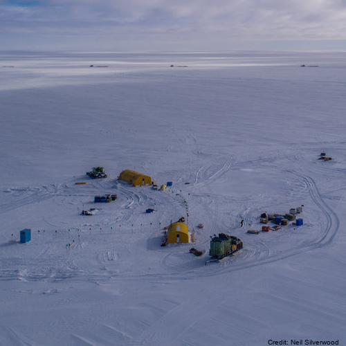
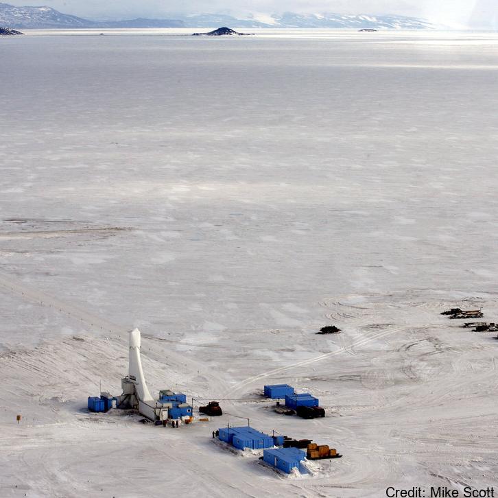
Here we provide data from the Ross Ice Shelf ocean cavity. The HWD2 Camp was established in October of 2017 at (-80 39.497, 174 27.678) where the ice is moving seaward at around ~600 m a-1 and is sourced from the Transantarctic Mountains. Profiling Instruments - Profiling was primarily conducted with an RBR Concerto CTD (conductivity-temperature depth) profiling instrument, and this was cross-calibrated against irregular profiles with an RBR Duet (pressure and temperature only), a SBE37 MicroCat CTD as well as moored SBE37 MicroCat CTDs. The RBR unit is small and has suitable sensor capability (temperature and conductivity accuracies of ±0.002°C and ±0.003 mS cm-1). Its conductivity cell design is not prone to fouling by ice crystals, making it ideal for work in the sometimes crystal-laden borehole conditions. We were inconsistent in how we mounted the CTD on its protective frame and this appeared to make small difference in the conductivity signal (resulting in an ~0.03 psu variation). This was post-corrected based on the essentially invariant mooring data from the lower water column as well as SBE37 cross-calibration profile data. Because of the potential for sediment contamination of the sensors, the profiles were mostly conservative in their proximity to the sea floor. On several occasions, profiles were conducted all the way to the sea floor. The temperature and salinity are presented in EOS-80 in order to compare with available data. Eighty-three profiles are provided here (ctd_HWD2_*.dat). In addition, limited microstructure profiling was conducted to provide insight into some of the mixing details. The profiles were conducted by lowering the instrument to the ice base then commencing a sequence of three up-down “yo-yos” before returning to the surface and downloading. A data segment is included here (VMP_HWD2.dat). There were some challenges registering the vertical coordinate for the profiles. The melting of the borehole generates a trapped pool of relatively fresh water. The interface between this and the ocean should be near the base of the hole or a little higher – with seawater intrusion. However, there were some instances where the interface was at a higher pressure (i.e. apparently in the open water column). The best explanation for this is that the water in the borehole is not at static equilibrium for some period after initial melting. We use 34.3 psu as a cut-off, in addition to a pressure criterion to identify the top of the useful oceanic profile. It is also not inconceivable that water was being ejected from the hole, but it is unlikely that this would have impacted in the consistent observed pattern. Instrumented Mooring - The mooring instruments at HWD2-A comprised 5 Nortek Aquadopp single point current meters in titanium housings reporting to the surface (30-minute interval, Table SI-Three) via an inductive modem to a Sound-9 data logger and Iridium transmitter. The current meter measurements were corrected to account for the 138° magnetic declination offset (i.e. the south magnetic pole is to the north-west of the field site). Five files are provided here (HWD2_Init_rcm*.dat4). Stevens Craig, Hulbe Christina, Brewer Mike, Stewart Craig, Robinson Natalie, Ohneiser Christian, Jendersie Stefan (2020). Ocean mixing and heat transport processes observed under the Ross Ice Shelf control its basal melting. Proceedings of the National Academy of Sciences, 117 (29), 16799-16804. https://doi.org/10.1073/pnas.1910760117

Ocean–atmosphere–sea ice interactions are key to understanding the future of the Southern Ocean and the Antarctic continent. Regional coupled climate–sea ice–ocean models have been developed for several polar regions; however the conservation of heat and mass fluxes between coupled models is often overlooked due to computational difficulties. At regional scale, the non-conservation of water and energy can lead to model drift over multi-year model simulations. Here we present P-SKRIPS version 1, a new version of the SKRIPS coupled model setup for the Ross Sea region. Our development includes a full conservation of heat and mass fluxes transferred between the climate (PWRF) and sea ice–ocean (MITgcm) models. We examine open water, sea ice cover, and ice sheet interfaces. We show the evidence of the flux conservation in the results of a 1-month-long summer and 1-month-long winter test experiment. P-SKRIPS v.1 shows the implications of conserving heat flux over the Terra Nova Bay and Ross Sea polynyas in August 2016, eliminating the mismatch between total flux calculation in PWRF and MITgcm up to 922 W m−2. RELATED PUBLICATION: https://doi.org/10.5194/gmd-16-3355-2023 GET DATA: https://doi.org/10.5281/zenodo.7739059